You need trading models, if you want to succeed as a trader on the long term. Trading systems are build on trading models. You trading system should be able to tell you when to buy and when to sell correctly something like 80% of the time.In the past two decades financial markets have changed drastically. Days of open cry pit trading are over. Electronic trading has replaced open outcry pit trading. All the stock exchanges in the world have become electronically and highly integrated with the other financial markets like the futures market and the currency market. Futures markets like Chicago Board of Options Exchange is one of the world’s largest futures and commodity trading exchanges. It is fully electronic. Did you read the post on how Ripple XRP made 22000% return in 2017. It entered 2018 above $1.9 but now is trading at $0.35. Cryptocurrencies are a rage among some day traders. Many forex brokers have now started offering cryptocurrencies. You can trade cryptocurrencies alongwith currencies.
Currency market is a decentralized over the counter market. It is also fully electronic. There is no central location for the currency market. It only exists on the computer networks. There is no central regulatory authority that controls the currency market. So currency market is infact a segmented market. A group of banks and big financial institutions can pool together and start doing business with each other. This created a segment in the market. There can be many segments in the market. As a result we can find different currency quotes in the different market segments. This is unlike the stock market that is regulated and offers the best price to customer by routed it to the location where the customer can get the best price.
Algorithmic trading is the rage now. Almost more than 80% of the trades that are being placed at NYSE are being made by algorithms. A rogue algorithm caused GBPUSD Flash Crash a few years back. GBPUSD fell almost 600 pips in a few hours in thin market hours during the Asian Market Session. This flash crash has been blamed on a rogue algorithm that had opened a big sell trade on the statement made by French President that Brexit will be hard for Britain. Flash Crashes are a constant danger now days. When a flash crash takes place stop losses don’t work as the market freezes and there is no one who is willing to take the buy side. You can read about the GBPUSD Flash Crash in detail in this post.
Security and Exchange Commission SEC is the regulatory authority that oversees the regulation of stock markets in USA. Currency market is not regulated so you won’t find the best quotes all the times. This also allows the brokers to play with your order at certain times. But in this post what we will be doing is building trading models that we can then use in algorithmic trading. Trading almost something like 80% of the trades are being placed by algorithms. These algorithms are watching the market 24/5. As a human you cannot watch the market 24/5. What’s the solution? If you cannot beat them, join them. Yes, learn algorithmic trading and start building your own algorithmic trading systems. If you are interested in learning how to use JAVA in algorithmic trading, I have developed a few courses on JAVA. First you should read this post on how to do algorithmic trading on Dukascopy JForex platform. If you are interested you can take a look at my course Java for traders.
Emotions Are Your Biggest Enemy in Trading
If you trade manually by looking at the charts, you are doomed from the start. Your emotions will in the end doom you. If you have opened a good trade, your emotions will tell you close it before the profit vanishes. So you close the trade listening to your emotions. After sometimes, you are shocked to see that the price continued in the right direction and now the profit is 200 pips. You had closed the trade for 50 pips profit too early. In trend trading, you need to ride the trend as long as you can. But your emotions will always force you to make wrong decisions. Most of the time you will close the trade too early. You will also keep the trade open too long when you should have closed it early. Only solution to getting rid of emotions is to develop a mechanical trading system that can be programmed. So that you get the signals and you then decide whether to take the trading signal or reject it. This is the only long run solution to avoid emotions.
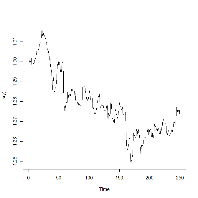
Above you can see the GBPUSD H4 price action plot. GBPUSD is notorious for showing unpredictable turns. You can see GBPUSD showing unpredictable turns in the above plot. Many day traders get burned when they try to trade GBPUSD. Developing a mechanical trading system is an interesting challenge. You test your mechanical trading system thoroughly on the demo account. This gives you a fair idea of how good it is in reality. Always remember, no trading system is 100% perfect. Every trading system will misjudge the market and give false signals. How to cater for that? You can cater for that by keeping the stop loss low something like 10-20 pips and try to catch the big moves that can make 100-200 pips. If you can do that your trading system does not need to have high winrate. A winrate of 50% will give you a profit of 500 pips in 10 trades on average if the average pips per trade are 100 pips. If you average stop loss is 15 pips, your average loss per 10 trades will be 150 pips. So your net profit will be 350 pips. So let’s try to develop a trading model that can predict the big moves in the market. If we can build such a trading model, we can then build a trading system based on that trading model.
Auto Regressive AR Trading Models
Auto regression is a statistical regression model in which we try to predict the future values based on the past values. This is precisely what we are doing when we look at the price chart and use it to predict the future price. Candlestick patterns are often used to predict the market turning points. But these methods based on candlestick patterns are vague and most subjective. Sometimes they work and sometimes they are simply wrong giving bad trades. We need a quantitative trading model that we can use to measure the success rate accurately. We will be using R and BUGS software to build Autoregressive models. You should be familiar with R. R is a powerful statistical and data analysis programming language. R is being used extensively at Wall Street. You should become familiar with R. When it comes to building Bayesian AR Models, we need Markov Chain Monte Carlo Simulation.
Above I said I have developed courses on how to use Java in building your algorithmic trading system. But the truth is R is the best language when it comes to do statistical modelling. Building robust algorithmic trading requires building good statistical models that can make the predictions that are reliable. R is perfectly suited for making statistical analysis. If you really want to master algorithmic trading, you should learn statistical analysis. You can read this post on fuzzy logic candlestick trading system using R.
In the past, it was difficult to do Markov Chain Monte Carlo (MCMC) Simulation. Bayesian modeling was not easy. We could only use simple models that had conjugate priors. Only those models that had conjugate priors were mathematically tractable. But in 1990s, computational power become cheap. With the tremendous increase in computational power at our disposal we can now do complicated modelling in just a few seconds. But BUGS software developed by Cambridge University made MCMC very easy. I will not go into the theory of MCMC. You should become familiar with Gibbs Sampling Algorithm and Metropolis Hastings Sampling Algorithm.
Developing a trading system is a process. What we need are good predictions. We need to take care of risk management and ideally have a small stop loss on average and a big take profit on average. You should be familiar with Reward/Risk ratio. We want a trading system that has at least 5:1 Reward/Risk ratio. If you have a good predictive statistical model, you can combine that with candlestick analysis and other technical analysis indicator and build a good predictive model. Read this post on a trading system that made 400 pips with a small 20 pip SL. 400 pips with 20 pips SL gives a Reward/Risk of 20:1 which is just fantastic. This happens when there is a rate announcement by the central bank.
Standard AR models use normal distribution as the error distribution. I will build an AR2 model with a Student T Distribution having one degree of freedom. It will take hardly a few seconds for the BUGS software to do the Monte Carlo Simulation and calculate the parameters of the models and then make the predictions. BUGS software was the catalyst that ushered in the Bayesian Revolution. So let’s start. First we read the data!
#BUGS modelling
source("G1.R")
# Import the csv file
data1 <- read.csv("D:/Shared/MarketData/GBPUSD240.csv",
                  header=FALSE)
colnames(data1) <- c("Date", "Time", "Open", "High", "Low",
                     "Close", "Volume")

#tranform the OHLCV data
#data3 <- newOHLCV(data1, 15)
#number of rows
#x1 <- nrow(data3)
x1 <- nrow(data1)
quotes1 <- data1$Close
#quotes1 <- data3$Close
#quotes1 <- data3$Low
#quotes1 <- data3$High
#quotes1 <- data1$Low
#quotes1 <- data1$High
#define k
k <- 1
y <- quotes1[(x1-250):(x1-k)]
In the above R code, we have read the GBPUSD H4 data. We will be using last 150 closing prices in predicting the next 10 closing prices. We will be using tsbugs R library to write the model. The parameters have uniform initial prior distribution. Variance of the model has got a gamma prior distribution. We have included 150 recent closing prices. The idea is to use data so that the model ultimately uses it to build the likelihood and then build the posterior distribution using MCMC (Markov Chain Monte Carlo).
> library(tsbugs)
> # AR(2) model with alternative prior
> ar2 <- ar.bugs(y, ar.order = 2, + ar.prior = "dunif(-20,20)",
var.prior = "dgamma(0.001,0.001)",
k = 10, sim = TRUE, mean.centre = TRUE) > print(ar2)
model{
#likelihood
for(t in 3:260){
        y[t] ~ dnorm(y.mean[t], isigma2)
}
for(t in 3:260){
        y.mean[t] <- phi0 + phi1*(y[t-1]-phi0) + phi2*(y[t-2]-phi0)
}
#priors
phi0 ~ dunif(-20,20)
phi1 ~ dunif(-20,20)
phi2 ~ dunif(-20,20)
sigma2 ~ dgamma(0.001,0.001)
isigma2 <- pow(sigma2,-1)
#forecast
for(t in 251:260){
        y.new[t] <- y[t]
}
#simulation
isigma2.c <- cut(isigma2)
for(t in 3:250){
        y.mean.c[t] <- cut(y.mean[t])
        y.sim[t] ~ dnorm(y.mean.c[t],isigma2.c)
}
}
Now this is an AR2 model with normal errors. We all know in financial markets, normal errors are rare. So I amend the above model code and use a student t distribution with one degree of freedom as the model errors. BUGS software comes in handy now. It can easily build the MCMC for estimating the posterior distribution when we have student t distribution errors. You might ask why use student t distribution and not normal distribution. Financial market has long tail data. Normal distribution does not has long tails. Student t distribution has long tails. I run the model now!
# Run in OpenBUGS
writeLines(ar2$bug, "ar2.txt")
library("R2OpenBUGS")
ar2.bug <- bugs(data = ar2$data,
inits = list(inits(ar2)),
param = c(nodes(ar2, "prior")$name, "y.sim", "y.new"),
model = "ar2.txt",
n.iter = 11000, n.burnin = 1000, n.chains = 1)
Now when I run this model, BUGS took just a few seconds to carry out 11000 iterations. First 1000 iterations were burn in and discarded. Just imagine 11000 interations were made within a few seconds. Below I give the predictions made by the AR2 BUGS model.
> ar2.bug$mean$y.new
 [1] 1.273498 1.274179 1.270601 1.269335 1.280929
1.280244 1.279322 1.280515
 [9] 1.273887 1.275194
> plot(ts(ar2.bug$mean$y.new))
As you can see these were the predictions made by the AR2 model for the next 10 H4 closing prices. You can see first GBPUSD price fell then it made a huge 100 pips move and then fell back. So our AR2 model can predict the big moves in the market.
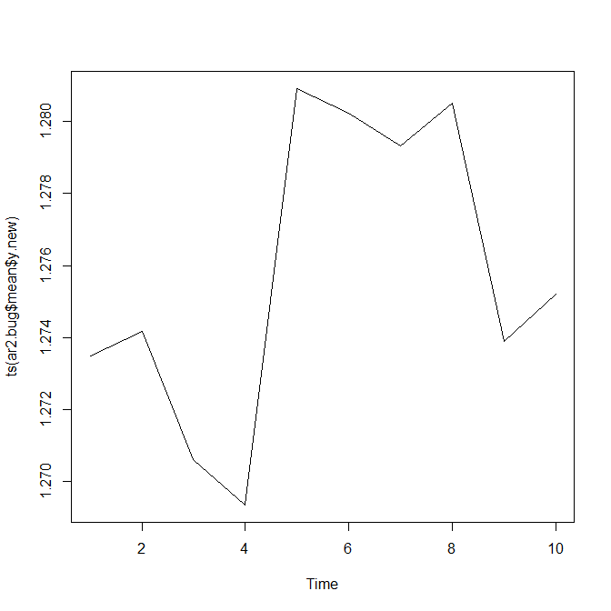
Above is the plot of the AR2 predictions!
# Plot the parameters posteriors and traces
library("coda")
param.mcmc <- as.mcmc(ar2.bug$sims.matrix[, nodes(ar2,
 "prior")$name])
plot(param.mcmc)
These are the plots of the posterior and the trace plot.
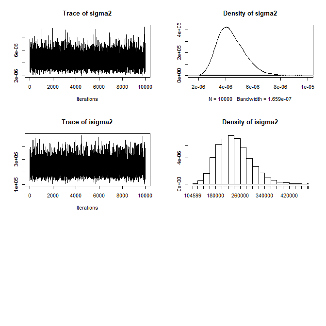
Above are the posterior distributions of the parameters and the trace plots. We can also build AR3 model and see if it is better. We can also build stochastic volatility models and see if we can use them in building our algorithmic trading system. Breaking news drives the currency market. We only have the Open High Low Close (OHLC) price to make the predictions in our algorithmic trading system. We know candlestick patterns can predict the coming market move. Our statistical analysis also confirms this when we use the closing price time series to make the predictions. Read the post on GBPUSD rally on early election news.
GBPUSD M30 AR3 MODEL
GBPUSD is under a lot of pressure due to Brexit. Yesterday UK Parliament rejected the government Brexit plan. Whenever a voting takes place on Brexit in the parliament, expect high volatility. If you have been using candlestick patterns in your trading, you know there are a number of candlestick patterns that are considered as good trend reversal or trend continuation signals. Some candlestick patterns are two stick patterns and some are three stick patterns like the evening star and the morning star patterns.So I think a third order AR model is best for predicting price. Let’s try a third order AR model below with student t errors. Student t distribution can much better model heavy tail behavior as compared to normal distribution.
> #BUGS modelling
> # Import the csv file
> data1 <- read.csv("D:/Shared/MarketData/GBPUSD30.csv",
+                   header=FALSE)
> colnames(data1) <- c("Date", "Time", "Open", "High", "Low",
+                      "Close", "Volume")
>
> x1 <- nrow(data1)
> quotes1 <- data1$Close
> #define k
> k <- 1
> y <- quotes1[(x1-100):(x1-k)]
> #plot(ts(y))
> library(tsbugs)
> #BUGS modelling AR3
> # AR(3) model with alternative prior
> ar3 <- ar.bugs(y, ar.order = 3,
+ ar.prior = "dunif(-20,20)", var.prior = "dgamma(0.001,0.001)",
+ k = 10, sim = FALSE, mean.centre = TRUE)
> print(ar3)
model{
#likelihood
for(t in 4:110){
        y[t] ~ dnorm(y.mean[t], isigma2)
}
for(t in 4:110){
        y.mean[t] <- phi0 + phi1*(y[t-1]-phi0) +
phi2*(y[t-2]-phi0) + phi3*(y[t-3]-phi0)
}
#priors
phi0 ~ dunif(-20,20)
phi1 ~ dunif(-20,20)
phi2 ~ dunif(-20,20)
phi3 ~ dunif(-20,20)
sigma2 ~ dgamma(0.001,0.001)
isigma2 <- pow(sigma2,-1)
#forecast
for(t in 101:110){
        y.new[t] <- y[t]
}
}
> library("R2OpenBUGS")
> ar3.bug <- bugs(data = ar3$data,
+ inits = list(inits(ar3)),
+ param = c(nodes(ar3, "prior")$name, "y.new"),
+ model = "ar3.txt",
+ n.iter = 11000, n.burnin = 1000, n.chains = 1)
[1] "guess attempt at initial values, might need to alter"
> ar3.bug$mean$y.new
 [1] 1.309031 1.308433 1.308448 1.308664 1.308947
1.312740 1.311597 1.310479
 [9] 1.309852 1.309153
> plot(ts(ar3.bug$mean$y.new))
Now as I said I have used student t distribution to model the while noise in the AR model. White noise means residuals that have zero mean. MCMC (Markov Chain Monte Carlo) is a powerful Bayesian Analysis technique that can estimate the parameters of the model and after fitting the model make predictions. Below is the plot of the predictions!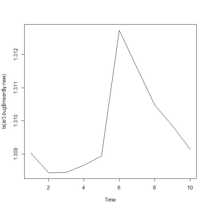
> tail(data1,10)
            Date  Time    Open    High     Low   Close Volume
16702 2019.01.30 09:00 1.30809 1.30952 1.30778 1.30862   1621
16703 2019.01.30 09:30 1.30861 1.30861 1.30670 1.30717   1348
16704 2019.01.30 10:00 1.30726 1.30934 1.30646 1.30893   2030
16705 2019.01.30 10:30 1.30892 1.31154 1.30892 1.31129   1800
16706 2019.01.30 11:00 1.31124 1.31215 1.31051 1.31082   1528
16707 2019.01.30 11:30 1.31081 1.31184 1.31050 1.31090   1085
16708 2019.01.30 12:00 1.31085 1.31162 1.30955 1.31011    952
16709 2019.01.30 12:30 1.31010 1.31148 1.30973 1.30977   1208
16710 2019.01.30 13:00 1.30980 1.31054 1.30870 1.31041   1222
16711 2019.01.30 13:30 1.31040 1.31042 1.30919 1.30920    493
Compare the closing price in the above OHLCV GBPUSD M30 dataframe with the model predictions above. Below is the GBPUSD M30 timeframe screenshot.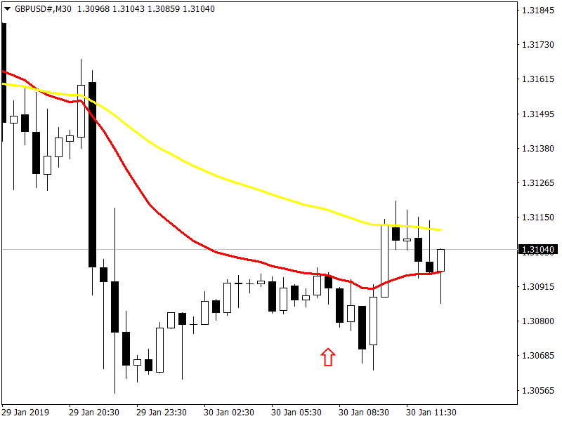
FOMC Meeting Predictions For GBPUSD
When I was updating this post, FOMC meeting was a few hours away. So I used the AR2 and AR3 models with student t distribution errors to make the predictions. Below is the screenshot of what happened during the FOMC Meeting.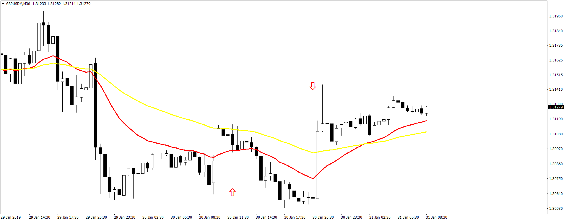
Model Comparison Using DIC
How do we know which model is better? If you have some idea about statistical modelling, you must have read about the AIC and BIC. AIC is the Akaike Information Criterion and the BIC is the Bayesian Information Criterion. DIC is Deviance Information Criterion. DIC is not an absolute measure. But it can be used to compare the models. The model having the lowest DIC is the better model.Unfortunately, in this case AR2 and AR3 both have a tie at around -1053. So what to do we can take the average of the observations. We need to keep our models simple. In the end, our results are only approximate.
> source("G1.R")
> data1 <- read.csv("D:/Shared/MarketData/GBPUSD30.csv",
+ header=FALSE)
> colnames(data1) <- c("Date", "Time", "Open", "High", "Low",
+ "Close", "Volume")
> ar3(data1)
 [1] 1.311065 1.310966 1.310493 1.312535 1.311044 1.313537 1.313031 1.313859
 [9] 1.314511 1.316374
> ar2(data1)
 [1] 1.310294 1.308912 1.308810 1.308753 1.302547 1.303160 1.302424 1.302366
 [9] 1.303582 1.307408
> 1.307408+1.316374
[1] 2.623782
> 2.623782/2
[1] 1.311891
> 1.311044+1.302547
[1] 2.613591
> 2.613591/2
[1] 1.306795
If we take the average of the two predictions, we have very good predictions. The second red arrow which is down in the above screenshot, it the time when FOMC Meeting Minutes were announced and GBPUSD shot up. The prediction has been made 5 hours earlier and is pretty good. So AR models are pretty good when it comes to predicting price. Just ensure that you are not using Gaussian white noise.
The above AR algorithms use MCMC (Markov Chain Monte Carlo) methods like the Gibbs Sampling and the Metropolis Hastings Algorithm at the back to do the parameter estimations and make the predictions. You should learn Bayesian Statistics and MCMC if you want to master price prediction using Bayesian AR Models. If you are interested in learning Bayesian Modelling for Algorithmic Trading, I have developed a few courses on that. In the next post, I am going to discuss Bayesian Stochastic Volatility Modelling and how we can use that in algorithmic trading.